
- Details
- Written by: Acacos
- Category: blog
- Hits: 590
Linear Regression, a cornerstone of data analysis, boasts a rich history dating back over a century. Introduced by luminaries like Francis Galton and Karl Pearson, its roots trace back to 1875 and 1920, laying the groundwork for concepts like Pearson Correlation.
While purists statisticians may debate its categorization within the realms of statistics rather than Machine Learning, let's not allow ourselves to become entangled in mere semantics. The true essence lies in its transformative potential, transcending disciplinary boundaries to become an integral part of the Machine Learning landscape.

Linear Regression: A Pillar of Machine Learning
But Linear Regression for puppies and bananas? Indeed, Linear Regression occupies a pivotal position within the realm of Machine Learning, offering predictive capabilities at its very core. Unlike traditional statistical approaches, Machine Learning algorithms adopt a forward-thinking strategy, leveraging data partitioning techniques by split the data into a training data subset, and a test subset to assess model performance proactively.
And the beauty of it all? Implementing Linear Regression is a breeze, whether it's a few lines of Python code or a series of keystrokes in Excel. Its accessibility underscores its relevance in the ever-evolving world of Machine Learning.
Delving Deeper: Unraveling the Science Behind Linear Regression
In this discourse, our focus transcends the mere execution of algorithms. Instead, we embark on a journey to unravel the intricate interplay of physical meaning, scientific underpinnings, and mathematical elegance. It's about more than just crunching numbers; it's about solving real-world problems with precision and finesse.
So, as we navigate through the complexities of Linear Regression, let's not merely scratch the surface. Instead, let's delve deeper, uncovering the profound insights and transformative potential that lie at the intersection of mathematics and artificial intelligence.
Mastering Linear Regression for Machine Learning
In our quest to harness the full potential of Linear Regression for Machine Learning, we embarked on a journey to explore three Python packages, each promising to deliver equivalent results and rival the capabilities of Excel. Let's delve into these 3 packages and unveil their unique features:
- Scipy: Linregress()
- Sklearn: LinearRegression()
- Statmodels: OLS()
While each of these 3 regressors boasts its own set of strengths and functionalities, determining the ideal choice boils down to personal preference and the specific nuances of the problem at hand. It's a decision shaped by context, not a one-size-fits-all solution. Notably, Scipy and Sklearn stand as stalwarts of Machine Learning and Artificial Intelligence, tailored to cater to the needs of modern data scientists. On the flip side, Statmodels OLS() caters more to the statistical community, offering a robust suite of tools honed over years of refinement.
Unveiling the Power of Linear Regression
Linear Regression, a cornerstone of curve fitting, holds a special place in my academic journey. During my graduate studies, I vividly recall its pivotal role in analyzing stimulus-response relationships, where independent variables (IVs) dictated the behavior of sensors, our dependent variables (DVs). With a graph in hand, predicting the response of any point within or beyond the measuring range became second nature. This extrapolation beyond the known realm, often termed forecasting, opened new vistas of understanding and insight.
Beyond the confines of academia, Linear Regression permeates our daily lives in subtle yet profound ways. From digital thermometers to velocity meters, fuel tank gauges to medical devices, the applications are myriad. It's the unseen force driving precision and accuracy, quietly shaping the world around us with every data point and prediction.
Real Life Datasets
In our journey through the realm of Linear Regression, let's start by delving into the heart of our analysis: the datasets. For the sake of simplicity and relatability, we've chosen datasets that mirror the activities we encounter in our daily lives. These datasets encapsulate metrics such as tips, order total amounts, and delivery fees from a restaurant, providing us with a rich reservoir of real-world with no human interference, so it is fair to assume no human error during the data collection process. With thousands of records at our disposal, we ensure the robustness and depth of our analysis.
Feel free to download the dataset and embark on this enlightening journey with us.
Unlocking Real-Life Scenarios
-
Business Services Expansion: Ever wondered whether it's more profitable to provide business services across 3 states or 2 states? ML hold the key to unraveling this conundrum, allowing us to dissect the financial implications of each scenario with precision.
-
Salesperson Strategy: Is it more lucrative to hire a salesperson to close 10 deals a day with a 12% premium, or close 14 times a day below the premium? Machine Learning offer valuable insights into sales performance metrics, enabling us to formulate data-driven strategies for maximizing revenue.
-
Delivery Radius Optimization: Should a food store manager offer a 5-mile, 3-mile, or 1-mile delivery radius? Through meticulous analysis of delivery logistics data, we can determine the most profitable delivery radius that strikes a balance between efficiency and customer satisfaction.
Decision Time: Which Short-Term Profit vs. Long-Term Branding?
As we navigate through these specific scenarios, we're faced with a critical decision: How do we balance short-term profitability with long-term branding objectives? Linear regression serves as our guiding compass, providing us with the analytical tools to make informed decisions that drive both immediate returns and sustainable growth.
Harnessing Linear Regression for Business Intelligence Strategy
Consultants and analysts leverage the power of linear regression to dissect real-world scenarios, extracting actionable insights and formulating robust business strategies. From optimizing sales tactics to fine-tuning delivery operations, linear regression empowers us to make data-driven decision that maximize profitability and propel business success.
Linear Regression Excel vs Python
When it comes to conducting Linear Regression analysis, both Excel and Python stand as viable options. However, it's crucial to understand the nuances and limitations of each approach. Let's delve into the comparison, focusing on the outcomes generated by Linear Regression using Excel and Python, and explore the implications for our analysis.
Excel Regression Output
-
Consistency in Results: The Linear Regression outputs obtained from Excel are expected to be consistent with those from Python. The ANOVA table provided by Excel offers a comprehensive overview of the regression analysis, laying the groundwork for further interpretation and analysis.
-
Limitations of Excel: While Excel serves as a convenient tool for basic regression analysis, it falls short in catering to the complexities of Machine Learning. Unlike Python, Excel lacks features such as data splitting and hyperparameter tuning, essential elements for robust Machine Learning models.

Navigating the Analysis
As we progress through this tutorial, we'll dissect and interpret the results obtained from both Excel and Python. By scrutinizing the strengths and limitations of each approach, we'll gain valuable insights into the practical applications of Linear Regression in Artificial Intelligence and Machine Learning. Stay tuned for a comprehensive exploration of regression analysis techniques and their implications for data-driven decision-making.
How to run the Linear Regression with Python Scipy?
Linear Regression analysis using Python's Scipy library offers a robust and efficient approach to extract meaningful insights from datasets. Let's dive into the step-by-step process of performing Linear Regression using Python, leveraging the Scipy library.
1. Set up the Data Frame with Pandas
- Pandas: Utilize the powerful Pandas package to create a structured data frame. Ensure that the CSV file containing the dataset has clear labels for easy organization and readability.
2. Extract Relevant Columns
- Data Extraction: Using Pandas, extract the necessary columns from the dataset. In this example, we focus on the "subtotal" and "tip" columns, which serve as the independent and dependent variables, respectively.
2. Extract Relevant Columns
- Data Extraction: Using Pandas, extract the necessary columns from the dataset. In this example, we focus on the "subtotal" and "tip" columns, which serve as the independent and dependent variables, respectively.
4. Perform Linear Regression
- Regressor Calculation: Utilize the stats.linregress function from Scipy to calculate the slope, intercept, correlation coefficient (r), p-value, and standard error of the regression model.
5. Evaluate Model Performance
- Coefficient of Determination: Assess the model's performance by calculating the coefficient of determination (R-squared) using the r2_score function from the
sklearn.metricsmodule.
6. Visualize the Results
- Data Visualization: Plot the raw data points, along with the training, testing, and predicted data points, using Matplotlib. This visualization provides a clear understanding of how well the Linear Regression model fits the dataset.
By following these steps, you can effectively run Linear Regression analysis using Python Scipy, enabling you to derive actionable insights and make informed decisions in the realm of Artificial Intelligence and Machine Learning.
import pandas
from scipy import stats

# Load Files & randmoize dataframe
df = pandas.read_csv('tipdata.csv')
df = df.sample(frac=1, random_state=42).reset_index(drop=True)

subtotal = df["subtotal"].values  # Independent Variable DV (X)
tip = df["tip"].values  # Dependent Variable IV (y)

# Split the data into train and test data
from sklearn.model_selection import train_test_split
subtotal_X_train, subtotal_X_test, tip_y_train, tip_y_test = train_test_split(
    subtotal, tip, test_size=0.5, random_state=42)

# The Regressor
slope, intercept, r, p, std_err = stats.linregress(
    subtotal_X_train, tip_y_train)

print("Slope:", round(slope, 3), " |  Intercept:", round(intercept, 2), " |  r:",
      round(r, 3), "|  P value: ", round(p, 5), "|  Std_Error: ", round(std_err, 3))

for tip_pred in tip_y_test:
    tip_pred = slope * subtotal_X_test + intercept

from sklearn.metrics import r2_score
Coef_Det = r2_score(tip_y_test, tip_pred)
print("Coef of Deter R-Squared:", round(Coef_Det, 3))

# Now lets plot the data
import matplotlib.pyplot as plt

plt.scatter(subtotal, tip, label='Raw Data')
plt.scatter(subtotal_X_train, tip_y_train, label='Train Data')
plt.scatter(subtotal_X_test, tip_y_test,
            label='Test Data', marker='*', alpha=0.3)
plt.scatter(subtotal_X_test, tip_pred, label='Predict Data', marker='.')
plt.xlabel("Subtotal")
plt.ylabel("Tip")
plt.title("Linear Regression for Machine Learning  \n")
plt.grid(color='gray', linestyle='--', linewidth=0.5)
plt.legend()
plt.show()
Optimizing Linear Regression with Python SciPy
In our quest for efficient Linear Regression analysis, we turn to the linregress function from the Python SciPy statistical package. Leveraging this powerful tool, we can streamline our analysis process and achieve robust results that stand the test of comparison against other widely used packages like Excel, R, or Java.
slope, intercept, r, p, std_err = stats.linregress(subtotal,tip)
Exploring the Output
The linregress function furnishes us with a comprehensive output, including the slope, intercept, Pearson coefficient (r), p-value, and standard error derived from the training data subsets. In our case, the dependent variable is the tip, while the independent variable is the subtotal.
It is easy to verify that the output of the linregress compares very well with the results shown in the Excel ANOVA table. Note, however, that the Excel output is for the whole data set of all the points while the linregress includes only half of the data for training the algorithm the other 50% is for testing the algorithm.
Slope: 0.13  |  Intercept: 0.83  |  r: 0.763 |  P value:  0.0 |  Std_Error:  0.002
Coef of Deter R-Squared: 0.623
Understanding Coefficient of Determination (R-Squared)
The coefficient of determination, often denoted as R-squared or R2, plays a pivotal role in assessing the predictive power of our model. When r is squared, we obtain the R-squared value, representing the proportion of the variance in the dependent variable that is predictable from the independent variable.
- First Coefficient of Determination (from the linregress train data): r to the power of 2 (0.763)2 = 0.582
- Second Coefficient of Determination (from the sklearn python library comparing the test data with the predicted values i.e. the tip_test data set vs tip_pred test data): 0.62
Both coefficients align closely with the Excel output of 0.604, showcasing the consistency and reliability of our analysis across different platforms.
Ensuring Clarity in Notation
To avoid confusion, it's imperative to maintain clarity in our notation. We distinguish between the Pearson Correlation Coefficient (r) and the Coefficient of Determination (R2) R-Square, or simply R2, ensuring precision in our analysis.
If we change the size of the train vs test subsets we will get slightly different results.
Examining the Scatter Plot
A visual inspection of the scatter plot reveals the presence of numerous outliers within our dataset, a phenomenon that warrants further discussion and analysis in subsequent stages of our exploration.
By harnessing the capabilities of Python SciPy and adopting a meticulous approach to our analysis, we equip ourselves with the tools necessary to conduct Linear Regression with confidence and precision in the realm of Machine Learning and Artificial Intelligence.

How to perform Linear Regression with OLS Statsmodel?
When it comes to Linear Regression analysis, leveraging the OLS (Ordinary Least Squares) library from Statsmodel is akin to wielding a precision tool in the realm of data science. Comparable to its counterpart, linregress, OLS offers a seamless pathway to unlocking insights from your dataset with unparalleled accuracy and efficiency.
Advantages of OLS Statsmodel
One of the standout features of OLS is its comprehensive summary report, a treasure trove of invaluable insights that provides a deeper understanding of your regression model. From coefficients to confidence levels, this built-in report is as close as it gets to Excel empowers analysts to glean actionable insights and make informed decisions with confidence.
Lets jump in the OLS regressor python code:
import pandas

# Load Files
df = pandas.read_csv('tipdata.csv')
df = df.sample(frac=1, random_state=42).reset_index(drop=True)

subtotal = df["subtotal"].values
tip = df["tip"].values

# Split the data into train and test data
from sklearn.model_selection import train_test_split
subtotal_X_train, subtotal_X_test, tip_y_train, tip_y_test = train_test_split(
    subtotal, tip, test_size=0.5, random_state=42)


import statsmodels.api as sm
# Do not forget to add the constant most of us do!
subtotal_X_train = sm.add_constant(subtotal_X_train)
model = sm.OLS(tip_y_train, subtotal_X_train).fit()
print(model.summary())

# Prediction method 1 with for loop
slope = model.params[1]
intercept = model.params[0]

for tip_pred_M1 in tip_y_test:
    tip_pred_M1 = slope * subtotal_X_test + intercept

from sklearn.metrics import r2_score
Coef_Det = r2_score(tip_y_test, tip_pred_M1)
print("Coef of Deter R-Squared Mthd_1:", round(Coef_Det, 3))


# Prediction method 2 with statsmodel predict fuction
subtotal_X_test = sm.add_constant(subtotal_X_test)
tip_pred = model.predict(subtotal_X_test)

Coef_Det = r2_score(tip_y_test, tip_pred)
print("Coef of Deter R-Squared Mthd_2:", round(Coef_Det, 3))
Interpreting Results
The summary report of the OLS model is displayed next, offering a comprehensive view of key parameters such as the slope, intercept, and coefficient. As demonstrated in the code, these crucial metrics can be effortlessly extracted programmatically, enabling analysts to delve deeper into the intricacies of their regression model.
Within the code snippet provided, we meticulously partitioned the data into training and test subsets, a fundamental step in ensuring the robustness and reliability of our analysis. Employing two distinct methods for predicting Y as a function of X—specifically, predicting the tip based on the subtotal—revealed a noteworthy consistency: both the custom loop function and built-in prediction methods yielded identical Coefficient of Determination values. This harmonious outcome underscores the precision and accuracy of the OLS regression model, reaffirming its efficacy as a cornerstone tool in the realm of data science.
.
                            OLS Regression Results
==============================================================================
Dep. Variable:                      y   R-squared:                       0.581
Model:                            OLS   Adj. R-squared:                  0.581
Method:                 Least Squares   F-statistic:                     4742.
Date:                Sun, 27 Feb 2021   Prob (F-statistic):               0.00
Time:                        00:59:50   Log-Likelihood:                -5227.2
No. Observations:                3416   AIC:                         1.046e+04
Df Residuals:                    3414   BIC:                         1.047e+04
Df Model:                           1
Covariance Type:            nonrobust
==============================================================================
                 coef    std err          t      P>|t|      [0.025      0.975]
------------------------------------------------------------------------------
const          0.8273      0.048     17.301      0.000       0.734       0.921
x1             0.1297      0.002     68.864      0.000       0.126       0.133
==============================================================================
Omnibus:                     1160.361   Durbin-Watson:                   1.970
Prob(Omnibus):                  0.000   Jarque-Bera (JB):            35288.718
Skew:                           0.989   Prob(JB):                         0.00
Kurtosis:                      18.621   Cond. No.                         63.5
==============================================================================

Notes:
[1] Standard Errors assume that the covariance matrix of the errors is correctly specified.

Coef of Deter R-Squared Mthd_1: 0.623
Coef of Deter R-Squared Mthd_2: 0.623
How to use Linear Regression with Python Sklearn?
Similarly, we wrote a quick code to model the dataset with the Sklearn LinearRegression package.
import pandas
from sklearn.linear_model import LinearRegression

# Load Files
df = pandas.read_csv('tipdata.csv')
df = df.sample(frac=1, random_state=42).reset_index(drop=True)

subtotal = df["subtotal"].values
tip = df["tip"].values

#Use Reshape otherwise headache errors
subtotal = subtotal.reshape(-1, 1)

# Split the data into train and test data
from sklearn.model_selection import train_test_split
subtotal_X_train, subtotal_X_test, tip_y_train, tip_y_test = train_test_split(
    subtotal, tip, test_size=0.5, random_state=42)

model = LinearRegression().fit(subtotal_X_train, tip_y_train)
tip_pred = model.predict(subtotal_X_test)

from sklearn.metrics import r2_score
Coef_Det = r2_score(tip_y_test, tip_pred)  # compare y test to y predict

print("Slope: ", round(model.coef_[0], 3))
print("Intercept: ", round(model.intercept_, 3))
print("Coef of Deter R-Squared: ", round(Coef_Det, 3))
The results from the Sklearn regressor are shown next. Sklearn does not provide a summary report like the OLS method, however, the coefficients could be either printed or data scientists could write their class functions. One quick comment is that the results of Sklearn compare very well with the other regressors we discussed in this article.
Slope:  0.13
Intercept:  0.827
Coef of Deter R-Squared:  0.623
Comparing Methods and Performance
So far we described 4 methods to run linear regression Excel, Scipy, OLS, and Sklearn. The advantage of one method over the others is subjective. In production, real life, depending on the situation machine learning experts need to run and compare all these methods, and based on needs (performance vs speed) someone could determine the best solution to solve their specific problem.
- For web applications, if Linear Regression is required for predictions, it might not be easily possible to use Excel. On the other hand, someone could easily call and run Python libraries.
- From the 3 Python Scipy, OLS, and Sklearn, it seemed that Sklearn compiled the regression much faster than the other libraries. Speed becomes more important as the dataset grows larger. During our trial runs, we used Eclipse with CPython however if speed is critical someone could use the PyPy it is estimated that PyPy is approximately 94 times faster, running similar code in just 0.22 seconds as opposed to 20 seconds. Again that is under specific large datasets conditions.
Understand Linear Regression Models
Linear Regression is a method that provides us with a linear model Y = β0+β1X+ε
Rearranged into Y = β1X+β0+ε
For the time being, we will ignore ε but must keep in mind that ε is of critical importance and it is called the error or residual!
Rewritten as Y = β1X+β0, this is nothing more than a linear function that was taught in 8th grade.
β1 is called the Slope
β0 is the Intercept
After substitution from the result and rewrite Y = (0.13)*X+$0.83 or $tip = 0.13($subtotal) + $0.83
So for each additional dollar in the ticket (subtotal), we expect a tip increase of 13 cents. Now, how about that $0.83? Many do not know how to describe the β0, that is why it is critical to understand the physical problem being solved. In this specific case, β0 is the opportunity loss with each delivery or lack of. Meaning instead of making the full amount which is the subtotal of the bill x 0.13 + $0.83, the driver is just making an average of $0.83 by sitting down and doing nothing. Also, note that with other datasets, the intercept β0 could be negative at which point the opportunity loss is clearer.
So to predict the tip associated with a subtotal of $25, we just substitute: $tip = (0.13)*$25+$0.83 = $3.25+ $0.83 = $4.08.
Understand Pearson Coefficient known as Correlation Coefficient
In our model, the Pearson Correlation Coefficient is 0.763. The Pearson Coefficient tells us how LINEAR is the co-relationship between a bivariate (X,Y), and is NOT how well the model fits the observation. Pearson Correlation Coefficient could be any number between 1 and -1.
- A Pearson Correlation Coefficient of zero means that there is no LINEAR relationship between the set.
- An ideal Pearson Correlation Coefficient of 1 or -1 means all the data in Y could be explained by a linear equation having a slope and an intercept where the error is zero.
So at 0.763 Pearson r, we could conclude that there is a good Linearity between our BiVariate, subtotal, and tip.
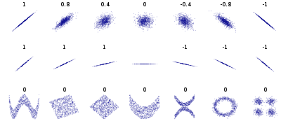
There are other correlation coefficients that we encourage you to read about from a textbook and understand. But in particular, is to practice and apply those correlations to real-life problems.
Assessing the Linear Regression model: Unveiling Performance Metrics?
In the realm of Data Science, the term "Good" is not absolute but comparative. A Good Model stands out by delivering superior performance when juxtaposed with its counterparts. To gauge performance effectively, a standardized metric becomes indispensable. Herein lies the significance of the Coefficient of Determination, commonly denoted as R-squared (R2).
Explanation of R square, Coefficient of Determination
R-squared, or the Coefficient of Determination, epitomizes the goodness of fit in statistical modeling. It elucidates the extent to which the variation in the Dependent Variable is elucidated by the Independent Variable. Linear Regression, being an optimization algorithm, endeavors to minimize R2.
In our scenario, R2 hovers around 60.04%, implying that 60.04% of the variance in Y (the tip amount) finds explanation in X (the subtotal of the delivery order). However, a pertinent question arises: What about the remaining 39.96%? Enter ε, the residual error term.
In Linear Regression, the Coefficient of Determination is computed as the square of the Pearson Correlation Coefficient. A complementary method yielding identical results is the ratio of the Sum Square of the Residual (SSR) to the Sum Square of the Total Error (SST). For instance, referencing the Excel output provided earlier, R2 is calculated as SSR/SST, where R2 = Regression / Total = 13382/22152 = 0.604119.
While this article delves into the fundamentals, advanced practitioners are encouraged to delve deeper into concepts such as SSR, SST, and SSE for a comprehensive understanding of model evaluation.
- Details
- Written by: Acacos
- Category: blog
- Hits: 510
Want to boost profits? It's all about mastering your product mix and menu engineering. Every business out there has a unique blend of products or services. But here's the kicker: survival hinges on meeting demand. Many managers fall into the trap of adding items willy-nilly until it's too late. Ever wondered why there's a labor shortage? Picture this: restaurants selling T-shirts and jewelry alongside gyros. Sounds bizarre, right?
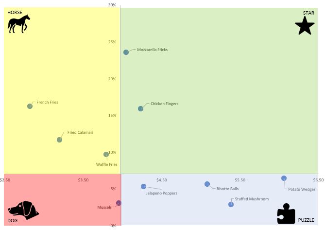
How to boost Profit using Product Mix & Menu Engineering
Enter product mix analysis, a game-changer since the '70s, pioneered by the Boston Consulting Group (BCG) with their Four Quadrants. Fast forward to '82, and at Michigan State University Michael Kasavana, Ph.D., and Donald J. Smith unveiled Menu Engineering, seamlessly merging product mix analysis with BCG's framework. Big players like McDonald's, Panera Bread, and Pizza Hut swear by it.
The product mix offered by any given Business is vital to success, kept unchecked it leads to failure.
- Too many items drain resources, leading to unnecessary costs like real estate, labor, and inventory.
- And watch out for Product Cannibalization—it's a real threat.
- On the flip side, too few offerings mean missed opportunities and lost profits.
Now, let's talk terminology. When we mention units sold, volume, popularity, or demand, we're talking about the same thing.
But here's the kicker: around 80% of the time, when we ask owners about their product mix, we get a laundry list. The savvy ones give us items with demand figures. The pros? They hand over lists with units sold and selling prices. Food costs? Rarely provided, and when they are, they're often ballpark figures. But hey, it's a start. For competitive analysis and strategy development, accuracy is key, especially with food costs.
Here's the golden rule: prioritize demand over margin. Why? Because demand is the cornerstone of branding and sets the stage for everything else. Profit? It's the endgame, a result of nailing demand, margins, and menu engineering. So, ready to take your profits to the next level? Stay tuned.
What is a Menu Engineering?
Restaurant Menu Engineering is like the secret sauce of maximizing restaurant profits. It's a slick strategy that falls under the umbrella of product mix analysis, leveraging operational data to make savvy decisions. But here's the kicker: it's not about ramping up sales; it's about slashing costs and beefing up that bottom line.
It is important to understand that Menu Engineering is a strategy to cut costs and boost profit. But it is NOT designed to increase sales.
Increasing sales is a different categorical strategy by itself. Upselling, cross-selling, and menu layout are some of the tools to increase sales. For instance, we tell clients to train their crew to offer deserts only after the order is finalized.
So, what's the deal with menu engineering? Think of it as a behind-the-scenes wizardry, where the layout and pricing of your menu are strategically orchestrated to entice diners without them even realizing it. Take desserts, for example. Ever notice how they're often offered after you've already ordered your main course? A well-presented dessert is difficult to resist. Sneaky, right? But effective.
Here's the playbook: front page, appetizers and mains. Second page? That's where the desserts lurk. It's all about guiding your customers through a tantalizing journey, one course at a time -Smooth, and Stealthy.
Looking for low-hanging fruits to cut costs? Then "menu engineering" should be on your top priority basket list!
But menu engineering isn't just some textbook theory you skim through and forget. It's a hands-on, trial-and-error process that marries item cost, units sold, and price point into a beautiful dance of supply and demand. And let's talk contribution margin. It's not about individual profits; it's about riding the wave of demand to maximize overall profit. Selling five (5) items with a $1 margin each beats selling two (2) items with a $1.50 margin, any day. Following demand is exactly at the heart of listening to the customer.
Before we explain further this "magic" formulation, we need to explain some psychological customer studies and powerful findings.
Limit Offering Choices (focus on profitable items)
Now, onto the psychology bit. Ever heard of the Paradox of Choice? It's the idea that too many options can actually paralyze decision-making. That's why streamlining your menu offerings can work wonders. Less is indeed More, my friend. So reduce offerings - You read it right!
Learning to choose is hard. Learning to choose well is harder. And learning to choose well in a world of unlimited possibilities is harder still, perhaps too hard.
– Barry Schwartz in his book The Paradox of Choice
Think about it: fewer buttons on a website (website conversion optimization), one sleek phone design instead of a dozen variations—simplicity sells. And in the world of menu engineering, simplicity means bigger profits. Ready to trim the fat and amp up your earnings? Menu engineering is your golden ticket.
Cas in point: did you notice that Samsung has several phone variations while Apple has one and only one phone design?
Apple Phones
- iPhone
Samsung Phones
- Galaxy S
- Galaxy A
- Galaxy Note
- Galaxy Ultra
- Galaxy Flip
- Galaxy Z Fold
Real-Life simple Menu Engineering case study
The best and easiest explanation of menu engineering is in the 20 oz Soda simple experiment. This is a real-life consulting service experiment we run for one of our customers. It has the Before and After numbers to measure performance. We run an experiment on 20 Oz beverages for a pizzeria. Beverages are commodities that are constant in flavor, and demand - sensitive only to cost.
Let's dive into a real-world case study that breaks down menu engineering in its simplest form: the 20 oz Soda Experiment. Picture this: a pizzeria facing the challenge of optimizing its beverage offerings. Sounds mundane, right? But the results are anything but.
Before we worked our magic, the lineup was pretty standard: 20 oz soda there was 6 flavors, nothing too fancy. But here's where it gets interesting. We ran the numbers, crunched the data, and pinpointed the sweet spot for maximizing profits. It's all about fine-tuning that product mix to hit the bullseye.
Product mix Before Menu Engineering Consulting
Before our menu engineering intervention in Q4 of 2017, the pizzeria offered a whopping six soda flavors. But here's the kicker: two (2) of them, the 20 oz Diet options, were absolute duds. Our matrix analysis revealed these underperformers, prompting us to nix them from the menu.
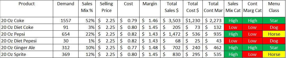
The matrix showed 2 Dogs the 20 Oz Diet offerings, we must stop selling these items.
The owner made some eye-opening observations. By ditching Sprite, they freed up space, downsizing from three (3) refrigerators to just two (2). Not to mention the hefty savings equipment maintenance. Oh, and let's not forget the headache of premature expiration—those diet sodas were notorious for going bad before they even hit the shelves.
Product Mix After Menu Engineering Consulting
Here is the product mix post-improvement Q4 of 2018, notice there are ONLY 3 flavors offered.
With a leaner menu in place, boasting just three soda flavors, the pizzeria saw a remarkable uptick in profitability. Despite slightly higher supply costs, the contribution margin soared from $4,380 to $4,727. Translation? An 8% profit boost. Sure, it fell short of our 15% target, but hey, a win's a win.
This case study underscores a fundamental truth: less is often more when it comes to menu engineering. By trimming the fat and focusing on high-demand items, you can unlock untapped profit potential. And for this pizzeria, the proof was in the soda—literally.
| Before Optimization | After Optimization | |
|---|---|---|
| Profit | $4,380 | $4,727 |
| Products | 6 | 3 |
| Fridges | 3 | 2 |
| Sales | $6,780 | $7,958 |
| Costs | $2,399 | $3,230 |
Boom!
High-five for nailing that Product Mix optimization! We've seen some serious wins across the board.
- Take a tire company we worked with—they slashed a cool $73,000 by kicking a sluggish tire brand to the curb. And that's just the tip of the iceberg.
- A mid-size retail chain? We steered them towards better-performing battery brands, pocketing a sweet $129,000 in savings. Talk about a win-win
Now, here's the kicker: you can rock the menu engineering game too. Too slammed to tackle it yourself? No sweat. Shoot us a message, and we'll whip up a quote faster than you can say "profit boost."
But here's the thing: optimization isn't a one-and-done deal. It's a journey, a continuous quest for improvement. That means keeping a finger on the pulse of your product lineup. When demand hits a plateau, it's time to shake things up with fresh offerings.
Sure, new products might start off slow, chilling in the "dogs" corner of the BCG quadrant. But hey, Rome wasn't built in a day. The key? Make 'em stand out, give 'em that competitive edge. And remember, a little cannibalism ain't so bad if it means long-term profitability. But if a new product's crickets, don't hesitate to cut it loose. Adaptation is the name of the game, my friend.
How to do Menu Engineering the easy way
Menu engineering isn't rocket science—it's a must-have tool for any food business, plain and simple. And guess what? The data you need is right there in your POS system, waiting to be unleashed.
1. Compile Your Data No need to reinvent the wheel. Just gather and update your existing data into a snazzy executive dashboard. Say goodbye to guesswork and hello to data-driven decisions.
Menu Engineering Categories
Let's break it down into four easy-peasy quadrants: As described earlier, menu engineering links demand with price and costs. Once you finish coupling price, demand, and costs, you need to classify these items into one of the 4 quadrant categories (Star, Puzzle, Horse, and Dog).
Stars: High Demand & High Margin.
Think of Stars as your menu's shining superstars. They're hot sellers with killer margins. Keep 'em front and center, no need for fancy promotions.
As the name implies, Stars are high profit, high popularity items. Relatively cheap to make, and customers can’t get enough of them - demand. These items must be extremely visible, top position on your menu, or a focal point with outstanding contrast and a quick call to action. These items must be kept consistent with no experimental variation. Should they be in advertising campaigns? Depends on your business goal and strategy but usually No —they're already fan favorites.
Puzzles: Low Demand & High Margin.
Puzzled by why these items aren't flying off the shelves? It's all about cracking the code. Puzzles are the items on your menu with a high margin, but the number of units sold is not enough. You are puzzled why you cannot sell more. Try to find out why they’re not selling — could they be better described or more prominently placed on your menu? Have you considered free samples or trained your crew to upsell? Promoted more on social media? Or, it might be that the price tag is a little too high. Sometimes, lowering prices slightly can increase popularity enough to induce higher profits. With Puzzles, margins are high and demand seems to be the problem. In such a case, more advertising makes sense, as long as it is part of the long-term branding strategy.
Horse: High Demand & Low Margin.
Horses are probably the easiest to fix pull up your TLC. These items are already established and popular so the only thing that requires maintenance is the margin. Almost the only option to fix this item is to reduce cost. Sourcing cheaper ingredients, buying bulk, and using this item as bait paired combos with a high margin item i.e. puzzle. Is there any leftover on customers' plates? Portion Control would be an acceptable answer. Is cooking time required? Save time and do not offer well done without request. Remember, these babies are in high demand, so every penny saved adds up.
Dog: Low Demand & Low Margin.
Ah, the dreaded dogs. Unlike their fluffy counterparts, these ones are more bark than bite. Most of the time, it's best to bid them adieu. Repairing these items? It's like trying to teach an old dog new tricks—costly and time-consuming.
Menu engineering doesn't have to be a headache. With a little know-how and some savvy strategy, you'll be boosting profits in no time. Ready to unleash the power of your menu? Let's do this!
Menu Engineering Essentials for Maximized Profit
Ready to dive into the nitty-gritty of menu engineering? Here's what you need:
- Analysis Time Frame
- Product Cost (this is a must!)
- Product Sale Price
- Units Sold (Demand)
- Categorize every Item into
- Star (High Demand, High Contribution Margin)
- Horse (High Demand, Low Contribution Margin)
- Puzzle (Low Demand, High Contribution Margin)
- Dog (Low Demand, Low Contribution Margin)
Analysis Time Frame
When diving into menu engineering, start by defining your analysis time frame. This isn't about how long it takes to do the analysis, but rather the period over which your sales data is collected. Think of it as segmenting your sales data into time series. Later, we'll explore how this helps pinpoint where each product stands in its life cycle
Product Cost
This step is make-or-break for your business's success. Yes, it's a bit of a grind at first, but getting your product costs spot-on is crucial. No more eyeballing it—conduct real tests, master portioning, and watch those costs fall into place. Don't forget to include labor costs and preparation time in your calculations. The variance in the cost due to portioning makes the food cost between 15% to 50%. Immediately after correctly running product costing many managers find hidden "leaks" and waste once they get this step right.
Product Sale Price & Units Sold
The data you need for this step is already at your fingertips, tucked away in your log files. But here's the kicker: don't overlook the details. Take into account discounts, promotions, and any other factors that might impact sales numbers.
How Often to Run Menu Engineering
Menu engineering isn't a set-it-and-forget-it deal. It's a dynamic process that requires regular attention. Here's a rundown of when to roll up your sleeves and dive back in:
The benefits of Menu Engineering go way beyond profit maximization it opens the managers' eyes to the dynamics of their business and gives them much-needed control.
Frequency of performing Menu Engineering:
- Before printing menus
- Prior to launching new items
- Before peak season hits
- After an economic crisis, inflation, long term supply prices increase
- At least once a year for a comprehensive check-up
By sticking to these guidelines, you'll keep your menu fine-tuned for maximum profitability. Ready to take your menu to the next level? Let's get started
Appetizers Menu Engineering Real-Life Example
Ever wondered what it takes to whip up a winning appetizer menu? Let's dive into a real-life case study that spills the beans. We had the permission to publish so here is a Real-Life Product Mix of restaurant appetizers after the 1st round of optimization.
Picture this: a jam-packed appetizer menu boasting a whopping 10 items. But here's the scoop—according to Miller's Cognitive Limitation, the sweet spot is 5 to 7 items. Why? Because our brains can only juggle around 7 items, give or take a couple. Keep it simple, keep it memorable.
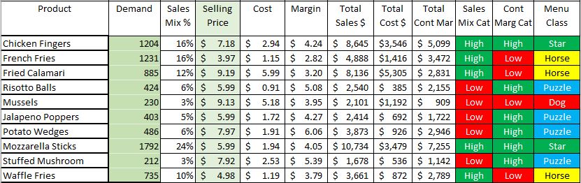
Menu Engineering Operations Optimization
Behind the Scenes Discussions
Now, let's peel back the curtain on some juicy discussions with our savvy customer:
- Calamari: A Horse with potential. How do we turn it into a Star? Easy—bump up the price by a mere 10 cents. Trust us, customers won't bat an eye, but your profits? They'll soar. Shoot for the stars with a price tag of $9.95 or even $10.45.
- Mussels: A Dog in disguise. Low demand, low margins—ouch. The verdict? Unless there's a compelling reason to keep 'em, they're out. But if you're dead set on keeping them, brace yourself for a makeover: jack up the price, trim costs (if possible), pump up the advertising, and fine-tune that recipe.
- Potato Overload: French Fries, Waffle Fries, Loaded Potato Wedges—talk about spud cannibalizing overload. Time to trim the fat. Can we consolidate? Pick one, maybe two at most. Both French Fries and Waffle Fries are Horses, meaning they're eating into each other's profits. Tough call, but a necessary one. Remember, a price increase is almost impossible as these are considered to be commodities.
And there you have it—the secret sauce to menu success. Menu engineering isn't just about tweaking prices or shuffling items around. It's about understanding the ebb and flow of your menu, anticipating customer cravings, and staying one step ahead of the game. That's why the best in the biz aren't just managers—they're leaders, charting the course for culinary greatness. Ready to join the ranks of the menu maestros? Let's make it happen.
Product Life Cycle
Ever pondered how products evolve over time? Let's peel back the curtain on the mysterious world of product life cycles. While there's a ton to unpack, we'll focus on the essentials to keep things crystal clear.
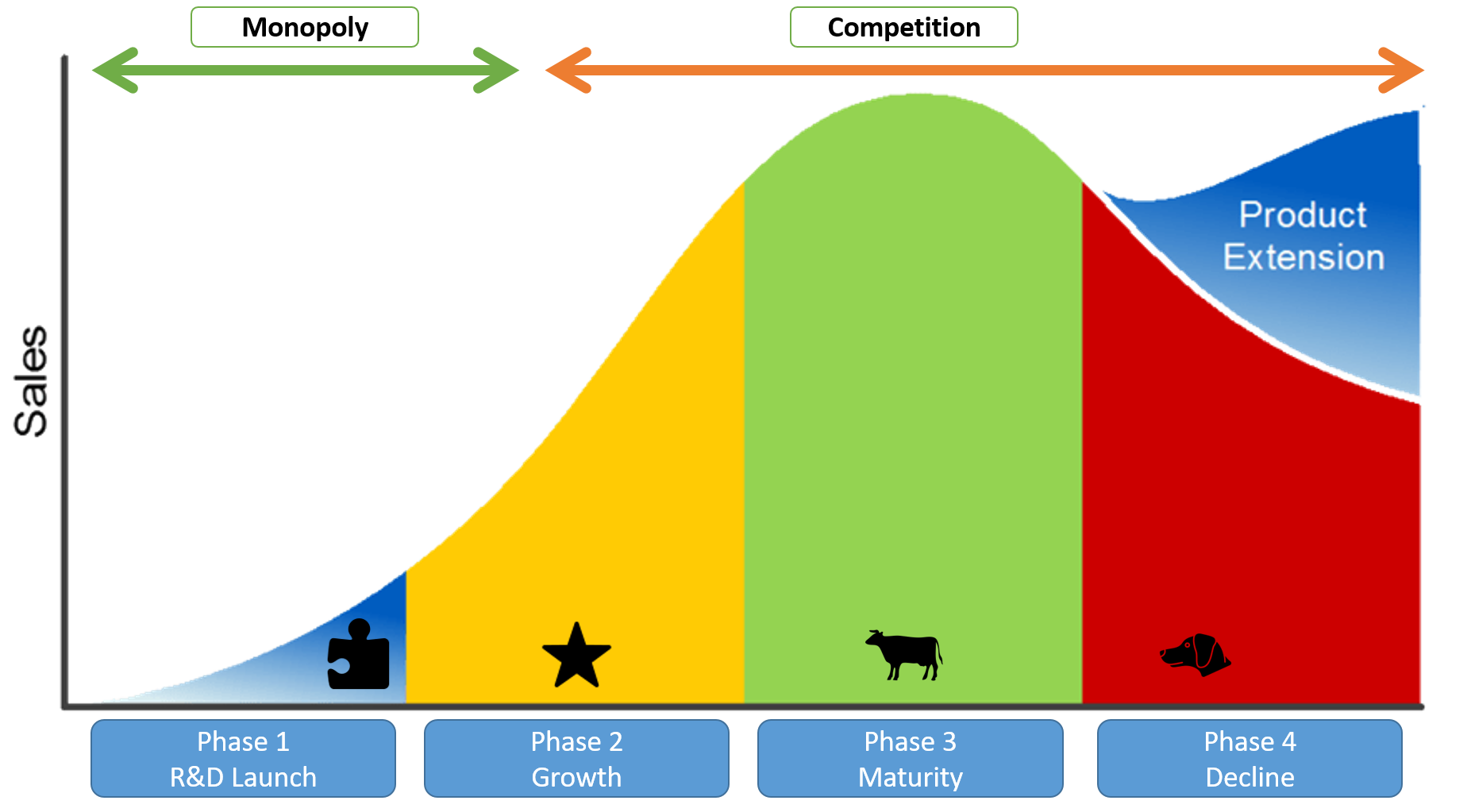
General Product Life Cycle Phases Curve
1. The Concept Unveiled
Picture this: the elusive product life cycle. It's a hot topic, with countless articles exploring strategies for each stage. But what's missing? A clear-cut mechanism to gauge where a product stands. We're here to shed light on this crucial concept, starting with the basics and promising a deeper dive in future articles.
2. Analyzing the Math Behind Growth
Now, let's zoom in on what really matters: spotting phase 2 growth products. Math might seem daunting, but fear not—we're breaking it down. First stop? Linear regression, and curve fit, and a little something called the Coefficient of Determination or R2.
Typically, during the initial introductory phase (1) a product must be fitted with a positive slope linear curve. After a given time frame, good marketing, and professional SEO campaign, if the product demand does not accelerate to a hockey stick (Shape) or exponential growth, then that product needs to be eliminated or re-engineered.
3. Deciphering the Data
Take a peek at our local pizza joint. We're comparing demand for Grandma (GM) and Margarita (Marg) pizzas. Both are served up under the same conditions to the same crowd. The verdict? Grandma's pizza steals the show, outselling Margarita by a landslide—4 to 1, to be exact.
But here's the twist: Margarita pizzas are cheaper to produce (much greater margin), yet Grandma's reigns supreme in demand. The secret sauce? Smart SEO tactics and strategic menu engineering. Grandma's pizza not only drives more sales but also boosts Customer Lifetime Value - Branding and Loyalty.
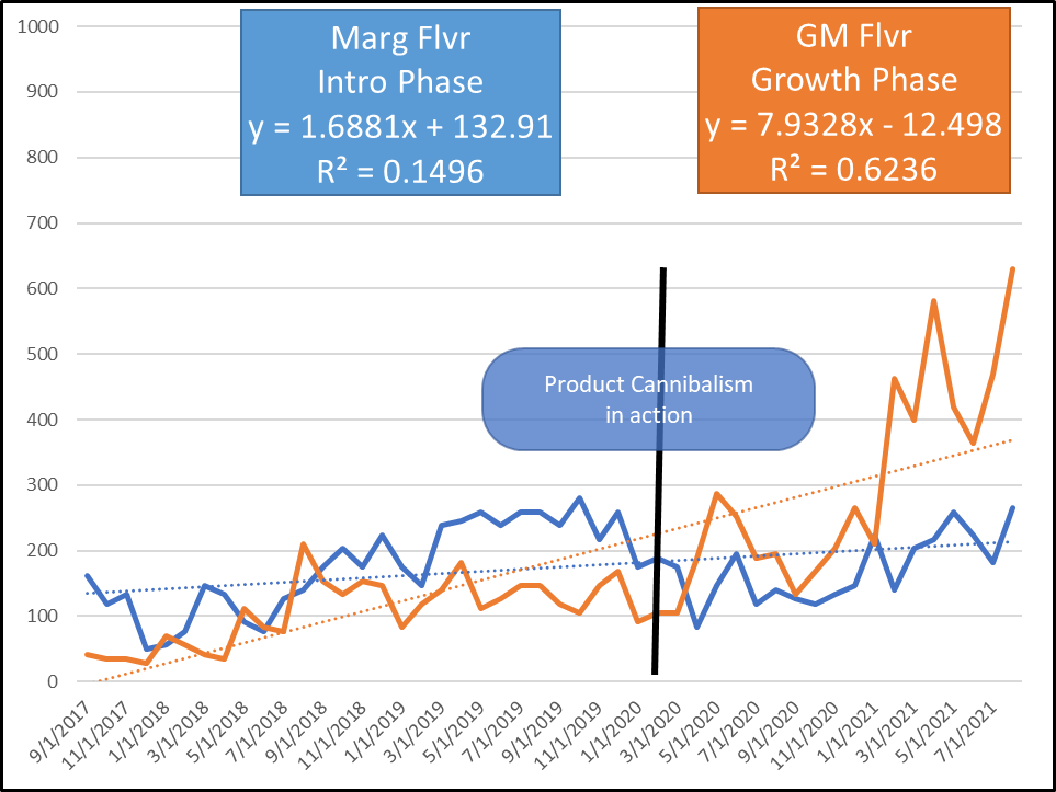
Product Life Cycle of Equivalent Products
Not finished yet, the graph also shows a real-life case of product cannibalism. Right where we draw the line, someone can see that while the owner was promoting the Margheritas the demand was slowly declining while the demand for the GM was picking up.
4. Growth Model Testing
We're not stopping there. We've put Grandma's pizza through the wringer, testing it against linear, 2nd order polynomial, and exponential growth models. The result? An exponential growth story with an impressive R2 value of 0.751—beating out even the mighty polynomial model. Talk about a star performer!
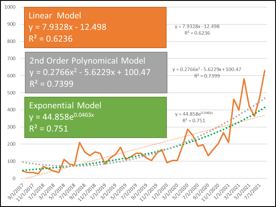
Product Life Cycle Growth Phase Equation
5. Business Intelligence Unveiled
Armed with robust mathematical evidence, we've crowned Grandma's pizza a menu engineering star and a BCG cash cow. But here's the kicker: this isn't just theory—it's real-world data, untainted by the COVID-19 pandemic's impact.
6. Charting the Course Ahead
Visionary business owners, take note: mastering these concepts is key to navigating the turbulent waters of business. Dashboards and algorithms are your compass, guiding you toward success. While these graphs were handcrafted, the future lies in automation—sorting through hundreds or thousands of products with ease.
- Details
- Written by: Acacos
- Category: blog
- Hits: 487
We will talk about small business owners in particular food shops and local restaurants. It strikes me that all these big thinkers do not have a consolidated order processing and accounting system, worse they still use pen and paper to process their orders. Here is my argument, every big company, McDonald, Panera, Starbucks, has a consolidated order processing and accounting system.
While searching for some food near me we found a pizzeria shop called Anthony's Pizza has been using Excel and Aldelo POS database to produce a full-blown weekly report, including, sales (from different food online portals such as UBER Eat, Grubhub, Delivery.com), drivers tips, employees hrs in about 10 minutes.
Data Automation with Excel
According to one of the owners, when they first started, generating weekly reports required over 12 hrs. Just do the math from 12 hrs/ week to just 10 minutes /week, for the sake of simplicity let's round off the saving to 11hrs/ week.
So 11hrs/ weeks x 52 weeks /year that's 572hrs /year.
If your business pays a dedicated person a minimum wage to compile these reports, that $572x$15/hr = $8550 annually - savings. If a bookkeeper with a rate of $20/hr performs the task the loss is apprximately $11,440pay.
What is the Best POS system?
While there is not such a thing as Best POS. Restaurant owners need to be in full control of their business and the first remote controllers are your POS and your accounting system.

We do not own, promote, or are involved with any POS company! This is not a disclaimer, this is a fact and here we are sharing our experience and what we learned. Here are our few tips if you decide to own a POS:
- Get a POS with a database that you could read and maybe edit
- Get a POS that is easy to use also easy to train crew members
- Get a POS that is fast and does not crash frequently
- Get a POS that is installed locally on the device and could run as a standalone without internet access. Should there be a requirement for the internet it should be only to sync with an external master database.
- Strongly recommended integrating the POS with an online ordering platform
There is an awesome article on how to install Unicenta on Linux / Ubuntu platform by Chubby and it works.
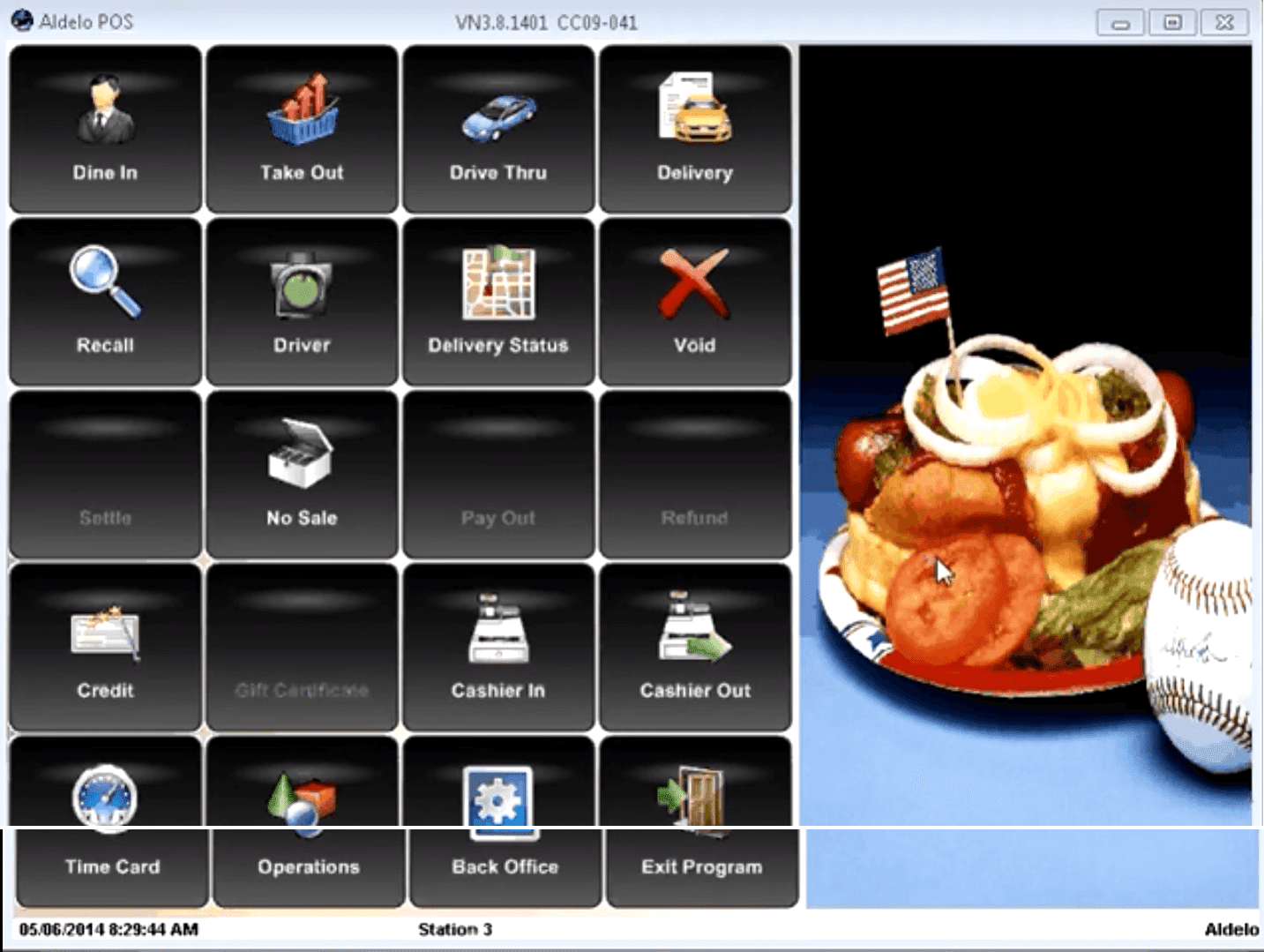
Aldelo pros
- It's locally installed and fast
- Orders on the screen are broken into Dine-In, Delivery, Take-out, and one more flexible config
- Well done access level - a cashier or junior level employee are limited to whatever the manager allows them to do.
- Native Loyalty Reward - but hold on
- Native Gift Certificate Program
- It easily handles bar codes
- It allows tables map
Aldelo cons - Yack! Really? The 2017 software release is the basis of our comments
- The worst thing about Aldelo, the user manual is so limited and not clear. Written for Aldelo representatives only - unless you attend a paid-for training and get certified, it is money down the drain.No online forum whatsoever!
- Support is "free" for 30 days only. Hold on. Once activated the support is available only for 30 days after that - they will milk you.
- It is still using an antique Microsoft Access Database with known corruption issues
- The loyalty Reward Program is a manual process. Need to ask the customer for their phone number every time to accumulate reward.
- The 2017 release screen resolution is limited to one size ONLY early 2000 era. It is NOT responsive.
- Two cities cannot share the same zip code.
- Who uses MapPoint in 2019? Pizzeria and restaurants live off local food delivery and MapPoint is so outdated and costs $300 for a license. Money that just went down the drain.
- Have you tried to configure a combo with Aldelo? A soup, a salad, and soda? Good luck! Luckily we were able to hear about tag-along items. And it simply does not work. And to get it up and running, you get charged.
- Calculation Errors
Aldelo Hacks | Excel Tips
Cross-network backup synchronization. Even better someone could use a powerful yet simple tool from samba utility this tool is called rsync and is very powerful to perform backups.
- Get time-resolved sales - Segmented
- Get menu item sales - Segmented if the software was set up correctly.
- Get customer sales and loyalty
- Get inventory reports
- Someone could develop a true Customer Life Value CLV. Aldelo has the elements to calculate CLV, but not enough to create an information-based decision. CLV is simply a priceless marketing metric - it is at the heart of a given business model. More about Customer Life Value.
- Someone could find the most profitable streets or delivery locations. With that, weaknesses could be identified and informed decisions could be made.
- How many consultants told you about menu engineering? Have you used Aldelo default menu engineering to realize how elementary it is? Does it provide value or help you make decisions? Do you have control over it?
Aldelo Menu Items Category
- Coffee
- Soft Drinks
- Wine
- Beer
- Pizza
- Entree
- Appetizers
- Salads
- Deserts
- Etc...
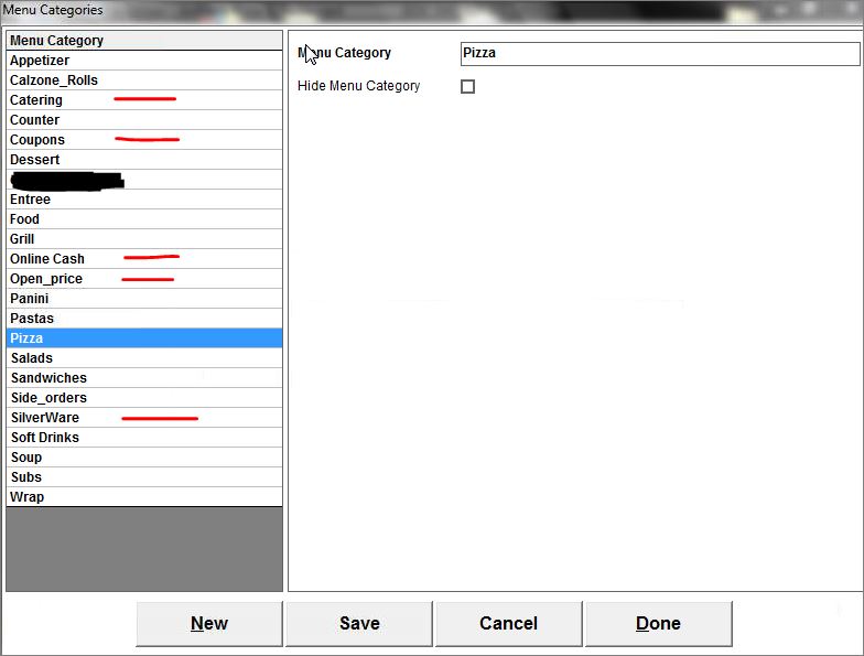
- Catering: This is used to segregate catering orders from large orders. Corporate Catering services is a recurring and profitable business, and owners could easily spot managers' effectiveness and their seriousness in getting catering business. Large orders, on the other hand, are random.
- SilverWare: This is equivalent to Utensils and used as a placeholder for $0 virtual menu items for delivery orders. Many hotel customers, order food from nearby pizzerias and request Plates, Forks, and knives. Guess what, the counter person who took the order forgot to write it down and the customer is upset and the driver did not get enough tips. So we added all possible utensils as menu items and dedicated a separate category. It helps when crew KIP are based on sales by dollar and menu items. In Hoboken NJ, the town started charging $0.10 for food take-out bags. Restaurants near Hoboken do not have to suffer through that non-sense additional tax.
- Coupons: We have to admit after trying to configure the discounts section of the Aldelo POS we failed miserably. Other than the basic percentage order or item discount or fixed dollar amount we could not do much. Documentation was not helpful so we decided to create our menu items and reverse engineer solutions that worked for us. Our combos, specials, and coupons all go to this Bin.
- Online_Cash: This is quite slick. Many restaurants get online cash orders. These cash orders unless entered into the system as cash transactions with an appropriate ticket #, payment for that order, either end up in someone's pocket or the cash register induces an over error. At the end of the night, the Manager could check all online orders and match them against this specific category.
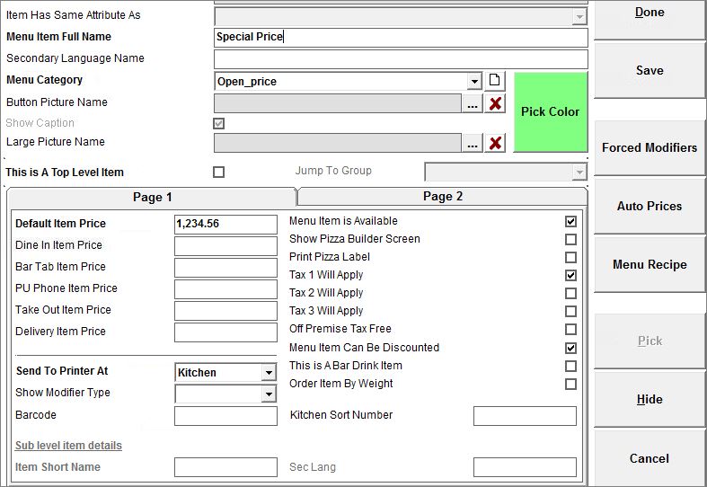
- Open_Price: This is equivalent to variable prices such as daily specials etc. In the Default Item Price just put 1,234.56. It is a catch-all for variable price items that are not in the printed menu. Here is the trick to having a variable price menu item on Aldelo. Noticed we categorized the variable price items under Open_price this helps trace errors, catch thieves and find items in demands that are not in the menu.
Excel For Aldelo
- Run Excel Pivot Tables (Power Pivot is a plus and could be used, Power Queries for Excel has some advantages and could handle very large datasets but as of 2019 standard Excel Pivot are easier and less buggy)
- Run Excel Queries (Power Queries is also an option but the files might be too large and take 1 minute to process and sometimes crush)